from_text_to_measurement
Source:vignettes/from_text_to_measurement.Rmd
from_text_to_measurement.Rmd
rm(list = ls())

library(dictvectoR)
library(dplyr)
library(fastrtext)
library(magrittr)
library(quanteda)
#> Warning in .recacheSubclasses(def@className, def, env): undefined subclass
#> "unpackedMatrix" of class "mMatrix"; definition not updated
#> Warning in .recacheSubclasses(def@className, def, env): undefined subclass
#> "unpackedMatrix" of class "replValueSp"; definition not updated
#> Warning in stringi::stri_info(): Your current locale is not in the list
#> of available locales. Some functions may not work properly. Refer to
#> stri_locale_list() for more details on known locale specifiers.

#> Warning in stringi::stri_info(): Your current locale is not in the list
#> of available locales. Some functions may not work properly. Refer to
#> stri_locale_list() for more details on known locale specifiers.
library(ggplot2)
Introduction
This vignette guides you through the workflow described in Thiele (2022) in applying the ‘Distributed Dictionary Representation’ (DDR) Method (Garten et al., 2018) and introduces most functions of the dictvectoR package.
The DDR method provides a continuous measurement of a concept in a dataset of documents. This measurement is obtained by calculating an average word vector representation of a concept dictionary, and representations of each document, and calculating the cosine similarity between those two vectors. For a detailed description, see Garten et al. (2018) and Thiele (2022).
Overview
The workflow described here starts from scratch, using only textual data as input, guides through steps for finding inductively a list of keywords, and demonstrates the evaluation and application.
It requires a population dataset containing textual data and a hand-coded sample drawn from this dataset, annotated for the presence of a theoretical concept. We use the built-in dataset tw_data as population data and tw_annot as annotated sample.
The vignette follows these steps:
Pre-process data
Train fastText model
Finding keywords
Add multi-words
Get F1 scores
Drop similar terms
Narrowing down by hand
Get combinations of terms.
Evaluate performance of combinations.
Apply best performing dictionary.
Face validity.
Pre-process data
First we load and pre-process the built in textual data.
clean_text cleans the text and is tailored to German-speaking texts on social media. If you are using text in other languages, you may want to adapt this helper-function to your own needs.
prepare_train_data prepares textual data for training a fastText model. It tokenizes longer documents into sentences, shuffles them, and calls clean_text with fixed settings.
We first prepare a texts character vector for training the fastText model, and clean the text in tw_data and tw_annot for our later analyses.
# Prepare text data
texts <- prepare_train_data(tw_data, text_field = "full_text", seed = 42)

# Clean text in tw_data
tw_data %<>% clean_text(remove_stopwords = T,
                        text_field = "full_text")

# Clean text in tw_annot
tw_annot %<>% clean_text(remove_stopwords = T,
                         text_field = "full_text")
Train fastText model
Now, we train our own fastText model using fastrtext::build_vectors.
A customized word vector model has the advantage that it maps the words and contexts that actually appear in the studied material. This is important here, as we will use the vocabulary of the model as starting point for our conceptual dictionary.
The downside of training your own model is that it is expensive regarding memory and computation. I used a machine with a CPU @ 1.80GHz processor with 8 cores and 16 GB RAM. If you run into memory limitations, consider decreasing dim, the number of dimensions. Decreasing the number of epochs will speed up the learing process, and decreasing the bucket size will reduce the size of the resulting model. For details, see Bojanowski et al. (2017). To obtain a model with better quality, you also should consider increasing the size of textual data used for training. The example here is limited by the size of data that can be feasibly shipped in a R-package.
Alternatively, you may consider using a pre-trained model from here.
The code below creates a local folder ft_model in your user home directory, and saves the model as two files: ft_model.bin and ft_model.vec.
(Note: To obtain a model that is reproducible every time we re-run the code below, we use only one core by setting thread = 1. To increase speed, you may want to use more threads.)
# Create local folder and set name for model
dir.create("~/ft_model", showWarnings = FALSE)
model_file <- path.expand("~/ft_model/ft_model")

# Train a fasttext model using the twitter data (if model does not yet exist)


  fastrtext::build_vectors(texts, model_file, modeltype = c("skipgram"),
                              dim = 150, epoch = 10, bucket = 1e+6,  lr = 0.05,
                              lrUpdateRate = 100, maxn = 7,  minn = 4, minCount = 3,
                              t = 1e-04, thread = 1, ws= 6)
 # }
Let’s load the model and use a nearest-neighbor query to check if it works properly. ‘Spahn’ is the name of the former German minister of health:
# Load model:
model_path <- path.expand("~/ft_model/ft_model.bin")
model <- fastrtext::load_model(paste0(model_path))

# Nearest-neigbor query:
fastrtext::get_nn(model, "spahn", k=8)
#>          spahns            jens   spahnversagen spahnruecktritt    maskenaffäre
#>       0.9231457       0.8296310       0.7667315       0.7490762       0.7094842
#>   maskenskandal        empfängt   ffpzweimasken
#>       0.7067993       0.7042576       0.6780393
Finding keywords
Next, we want to use the fastText model and the manually annotated dataset to find a short dictionary for populist communication.
First, we split the annotated data into a train and a test sample, using caret::createDataPartition.
# set seed
set.seed(42)

# get index for splitting
train_id <- caret::createDataPartition(tw_annot$pop,
                                times = 1,
                                p = .7,
                                list = F)
# split annotated data
df_train <- tw_annot %>% slice(train_id)
df_test <- tw_annot %>% slice(-train_id)
As starting point for our dictionary, we use the vocabulary from the fastText model. We add the ID from the vocabulary and use clean_text to remove stopwords, and drop words of less than 3 characters from this list:
# # Get vocabulary
vocab_df <- fastrtext::get_dictionary(model) %>% data.frame(words = .)

# Get vocabulary ID
vocab_df$word_id <- fastrtext::get_word_ids(model, vocab_df$words)

# remove stopwords
vocab_df <- clean_text(vocab_df,
                       text_field = "words",
                       remove_stopwords = T) %>%
            filter(n_words == 1,
                   n_chars > 2)
Next, we want to narrow down that list. We identify words that are similar to the hand-coded corpus of populist Tweets but dissimilar to non-populist Tweets in df_train using find_distinctive.
find_distinctive computes an average representation of that subset of the annotated corpus in which populism was coded as present, as well as a representation of the negative counterpart, i.e. of the non-populist corpus. It then computes the cosine similarities of each word in a dataframe to these two corpora, and calculates the difference between these two similarity scores. This provides us with a quick and computationally inexpensive shortcut to find keywords that capture a specific concept, but nothing else.
# Get distinctive word scores
vocab_df <- find_distinctive(df_train,
                             concept_field = "pop",
                             text_field = "text",
                             word_df = vocab_df,
                             word_field = "words",
                             model = model)

vocab_df %<>% mutate(pop_distinctiveXpossim = pop_distinctive*pop_possim) %>%
              filter_ntile("pop_distinctiveXpossim", .75)
However, this method of narrowing down a list of keywords is a bit crude and not very informative for assessing how well a single word would perform when used in the DDR method.
Hence, we want to get the actual F1 scores for each single word, when used as a one-word-dicitonary in the DDR method. Note that the DDR method returns the cosine similarity as a continuous measure, theoretically ranging from -1 to +1, while our manually annotated dataset was coded in a binary fashion (populist or non-populist).
To solve this problem, the continuous measure is used as a independent variable in a logistic regression, predicting the manual binary coding. To obtain Recall, Precision and F1 scores, dictvectoR compares the binary predictions resulting from this regression with the manual coding. This is not a direct gold standard test but circumvents the problem of producing reliable granular codes manually (Grimmer & Stewart, 2013, p. 275).
Recall is an evaluation metric that indicates how well the automated measure captures all true positives, precision is indicates how well it captures only true positives, and F1 is a harmonic mean of both (Chinchor 1992).
get_many_F1s is a function that efficiently returns F1 scores for a list of words or dictionaries, when used in as dictionary in the DDR method.
vocab_df$popF1 <- get_many_F1s(vocab_df$words,
                              model = model,
                              df = df_train,
                              reference = "pop")
We’re only interested in the best-performing quartile, which we extract using the helper-function filter_ntile:
top <- vocab_df %>%
            filter_ntile("popF1", .75) %>%
            filter(popF1 > 0)
Add multi-words
Some concepts are expressed rather in multi-word expressions than by single words. In our case, we suspect that people-centrism, one core dimension of populism, may involve such multiword expressions, for example by constructing an in-group with references to some ‘we’, e.g., ‘we taxpayers’, ‘our land’ etc.
To find common multiword expressions, we use the population data (that is 75 percent of it to speed up the process a bit), and tokenize it using quanteda::tokens.
tw_data %<>% filter(n_words >= 2)

# Use 75% sample
set.seed(42)
tw_split <- tw_data %>% slice_sample(prop = .75)

# tokenize
toks <- quanteda::tokens(tw_split$text)
add_multiwords adds multiword expressions for a dataframe of single words and counts the occurences. Here we only look for multiwords in a 2-word-window (level = 1), which can be increased to a 3-words window (level = 2). This process might take two or three minutes.
top <- add_multiwords(top,
                      tokens = toks,
                      min_hits = 1,
                      word_field = "words",
                      levels = 1)
#> [1] "Finding multi-word expressions in window = 1..."
#> Joining, by = "from"
#> [1] "Adding missing count of original words:"
#> [1] "Counting word occurrences..."
We want to narrow down this list again, dropping terms that occur only once. And we add a unique word_id by add_word_id.
top %<>% filter(hits > 1)
top %<>% add_word_id()
Get F1 scores
Now, we also want to know the F1 scores for the new multiword terms, hence we just run get_many_F1s again.
top$popF1 <- get_many_F1s(top$words,
                          model = model,
                          df = df_train,
                          reference = "pop")
Drop similar terms
The resulting list of words is quite long and includes a lot of redundancy. Note that unlike in traditional dictionary approaches, the DDR method performs better if the input dictionary is very short and clear-cut. While redundancy is not a problem for traditional dictionaries, it may distort the performance of the dictionary in DDR (Garten et al., 2018).
remove_similar_words helps us to detect similar terms - by computing the pairwise cosine similarity between all words representations in a datafram. It can use two score as input to decide which words to drop: Here we use the F1 score calculated before popF1, and the number of occurences (compare_hits = T). We set the function to compare only terms that reach a smiliarity of 60% (min_simil = .6). win_threshold defines the share of all comparisons that a term must win in order to remain in the dataframe.
Additionally, we drop terms that originate from the uni-word afd, the German populist party, since we want our populism measure to be rather non-partisan:
## narrow down
top_subs <- top %>% remove_similar_words(model,
                                        compare_by = "popF1",
                                        compare_hits = T,
                                        min_simil = .6,
                                        win_threshold = .5) %>%
                    filter(!from == "afd")
#> Warning in .recacheSubclasses(def@className, def, env): undefined subclass
#> "unpackedMatrix" of class "mMatrix"; definition not updated
#> Warning in .recacheSubclasses(def@className, def, env): undefined subclass
#> "unpackedMatrix" of class "replValueSp"; definition not updated
Narrowing down by hand
Let’s have a look at all terms found so far. (We won’t print all 400 or so terms here but only the top 50)
top_subs %>% arrange(desc(popF1)) %>% pull(words) %>% head(50)
#>  [1] "panzer"                 "örr"                    "verrechnet"
#>  [4] "örr zwangsgebühr"       "deutschen steuerzahler" "existenzen vernichtet"
#>  [7] "wand"                   "autofahrer"             "gaga"
#> [10] "wahn"                   "irrsinnige"             "rücken wand"
#> [13] "irrweg"                 "vernichtet"             "rechnet"
#> [16] "bargeld"                "merkels groko"          "kette"
#> [19] "lobbyregister"          "vdk"                    "deckmantel"
#> [22] "mdb groko"              "gender gaga"            "deckt"
#> [25] "autofahren"             "diesel benziner"        "groko plant"
#> [28] "entlarven"              "steuerzahler"           "teure"
#> [31] "abgasnorm"              "benziner"               "daimler vw"
#> [34] "palmöl"                 "seehofer rechnet"       "kleinrechnen"
#> [37] "deutschen mittelstand"  "groko importiert"       "skandalösen"
#> [40] "betreiber"              "mdb nimmt"              "spahn warnt"
#> [43] "unfähig"                "deutsche steuerzahler"  "todesstoß"
#> [46] "zwangsgebühr"           "teures"                 "verrückt"
#> [49] "geld deutschen"         "steuergelder"
This list of keywors is still quite long. It includes many terms that seem theoretically plausible, but also many words that obviously are either too specific, or seem out of place.
Since the next steps involve combinatorics for finding a good combination of keywords, we want to narrow down the list of words as drastically as possible.
For theoretical reasons, we decided to group the found words in three categories that reflect different aspects of populist communication: Terms that reflect ‘elites’, terms that reflect ‘the people’, and words that relate those two groups.
From the 400 or so terms, we hand-picked five distinctive terms for each of these categories. This mode of selection is theory-driven and different from the inductive logic used so far. You may want to opt for different modes of selection, depending on your task and the quality of inductively generated keywords. Here are the words picked for further processing:
elites <- c(
"altparteien",
"lobby",
"merkels groko",
"regierungsversagen",
"zwangsgebühr"
)

people <- c(
"arbeitnehmern",
"deutschen steuerzahler",
"existenzen vernichtet",
"mittelstand",
"volkes"
)

relation <- c(
  "irrsinnige",
  "entlarven",
  "skandalösen",
  "unfähig",
  "realitätsfern"
  )
We use this hand-picked list of words to create a shortlist and add a variable that indicates the category:
top_elites <- top_subs %>% filter(words %in% elites) %>% mutate(cat = "elites")
top_people <- top_subs %>% filter(words %in% people) %>% mutate(cat = "people")
top_relation <- top_subs %>% filter(words %in% relation) %>% mutate(cat = "relation")

shortlist <- bind_rows(top_elites, top_people, top_relation)
shortlist$cat %<>% factor()
shortlist$cat %>% summary()
#>   elites   people relation
#>        5        5        5
Get combinations
We now use this shortlist to get all possible combinations of various length per category, and all possible combinations of these combinations.
get_combis helps us finding these combinations, and provides a useful random sampling mechanism that limits the number of returned combinations: Setting a limit, limits the number of combinations of a given length returned per dimension.
For example, consider that you have a shortlist of words with 2 categories A and B, with 10 words per category, and want find combinations of words that include at least 3 words per category (min_per_dim = 3) and maximum 10 words overall (max_overall = 10), i.e. max. 5 words per dimension.
Then you would have 120 possible combinations of length 3 for both category A and B:
However, you also get 210 possible combinations of length 4, and 252 combinations of length 5 per category:
If you want to get all possible combinations of these combinations, the number increases really quickly, as we can see below. The first two lines return all possible cominations for A and B of varying length between 3 and 5. expand_grid returns the combinations of combinations:
A_c <- do.call("c", lapply(3:5, function(i) combn(A, i, FUN = list)))
B_c <- do.call("c", lapply(3:5, function(i) combn(B, i, FUN = list)))
expand.grid(A_c, B_c)  %>% nrow()
#> [1] 338724
Setting the limit to, let’s say 30, in get_combis radomly draws only 30 possible combinations of one length per category.
In our case, this limit is not really necessary, as we only have 5 words per category and want lengths between 3 and 4. The maximum number of combinations per length & category is 10:
Although unnecessary in our case, we specify a limit (that won’t drop any combinations) - just for demonstration. Setting seed makes your results reproducible, the default is 1. get_cobmis returns a data.frame that includes a column where you’re settings are stored, in case you want to come back and draw a different round of combinations.
So, let’s get all combinations for our list of words:
combis_rd <- get_combis(shortlist,
                        dims = "cat",
                        min_per_dim = 3,
                        max_overall = 12,
                        limit = 10,
                        seed = 42)
#> Joining, by = "rowid"
Evaluate combinations
Now we want to get Recall, Precision, and F1 scores for all of the 3,375 combinations. get_many_RPFs is made for this task:
combis_df <- get_many_RPFs(keyword_df = combis_rd,
                             keyword_field = "combs_split",
                             model = model,
                             text_df = df_train,
                             reference = "pop",
                             text_field = "text")
#> Joining, by = "rowid"
Now, let’s pick the best performing short dictionary:
# Pick dictionary that maximizes F1:
dict  <- combis_df %>%
          filter(F1 == max(F1)) %>%
          pull(combs_split) %>%
          unlist()

# Let's see:
dict
#> [1] "altparteien"            "deutschen steuerzahler" "existenzen vernichtet"
#> [4] "irrsinnige"             "mittelstand"            "regierungsversagen"
#> [7] "skandalösen"            "unfähig"                "zwangsgebühr"
These 10 words nicely cover various aspects of populist communication. However, this is not the place to dive into theoretical discussions.
Let’s check the performance of the dictionary instead. On the training sample, this dictionary reaches an F1 of .55, which is not great, but OK.
Let’s check the F1 score when applied on the test sample:
# Performance for test_df
get_F1(df_test, dict, model, 'pop')
#> [1] 0.4791667
The short dictionary reaches a F1 of .48 in the test sample, which is a somewhat weaker performance than in the train data.
For a real application, this might be considered a too weak performance. Pathways to improve this performance are discussed in the concluding section. Please note that the purpose of this vignette is not to demonstrate the performance of the DDR approach, but to introduce the functions of the package which can be used to enhance this performance.
For some applications, you might be interested about how your DDR measurement performs in different subsets of your data, e.g., if you are using a translated corpus originating from various languages. F1 scores for grouped subsets of a text-dataframe, can be obtained by get_many_F1s_by_group.
In our example, we might be interested in finding a dictionary that performs well for predicting populist communication of different political parties. Here, we demonstrate the function using the top 5% of short dictionaries. We focus on the overall performance, and the performance in predicting populist communication for the right-wing and left-wing populist parties AfD and Die Linke. We calculate the 3rd root of the product of the overall F1 score and the two party-specific F1-scores to pick the best performing ‘balanced’ dictionary:
combis_subset <- combis_df %>% filter_ntile("F1", .95)

combis_df_by_group <-  get_many_F1s_by_group(keyword_df = combis_subset,
                                             keyword_field = "combs_split",
                                             id = "id",
                                             model = model,
                                             text_df = df_train,
                                             group_field = "party",
                                             reference = 'pop')
#> Joining, by = "id"
# Compute 3rd root product of 3 F1s:
combis_df_by_group %<>% mutate(F1_balanced = (F1*F1_AfD*F1_Linke)^(1/3))

dict_bal  <- combis_df_by_group %>%
                        filter(F1_balanced == max(F1_balanced)) %>%
                        pull(combs_split) %>%
                        unlist()

dict_bal
#>  [1] "arbeitnehmern"          "deutschen steuerzahler" "existenzen vernichtet"
#>  [4] "lobby"                  "merkels groko"          "mittelstand"
#>  [7] "realitätsfern"          "skandalösen"            "unfähig"
#> [10] "zwangsgebühr"
Let’s check the performance of this ‘balanced’ dictionary on the test data:
get_F1(df_test, dict_bal, model, 'pop')
#> [1] 0.4948454
This more balanced dictionary performs slightly better in the test sample. Also, it drops keywords that are more or less exclusively used by the right-wing AfD, like ‘altparteien’ (translated: ‘old parties’).
Apply DDR
Having decided on a final dictionary, we want to apply this dictionary using the DDR method to the datasets. We apply it on both, the population data tw_data and the annotated data tw_annot, using the core function of this package cossim2dict. This function can also fill in missing values, which occur sometimes if text cleaning empties the text field. Here, we fill it by the mean minus 1 SD:
tw_annot$pop_ddr <- cossim2dict(df = tw_annot,
                               dictionary = dict_bal,
                               model = model,
                               replace_na = 'mean-sd')

tw_data$pop_ddr <- cossim2dict(df = tw_data,
                               dictionary = dict_bal,
                               model = model,
                               replace_na = 'mean-sd')
Face validity
Now, lets inspect the top 6 populist Tweets in our population data:
tw_data %>% arrange(desc(pop_ddr)) %>% pull(full_text, party) %>% head()
#>                                                                                                                                                                                                                                                                                              Linke
#>     "#Scheuer ist als Minister unfähig & untragbar! Vom PKW-Maut-Desaster über ÖPP-Straßenprojekte bis zur Autobahn GmbH: Wie lange will #Merkel noch zusehen, wie unser Steuergeld für private Beratungsfirmen, Investoren und überbezahlte Manager veruntreut wird? https://t.co/4x0a2UhuIh"
#>                                                                                                                                                                                                                                                                                              Linke
#> "Grotesk: #Lufthansa-Führung erpresst Beschäftigte mit Stellenabbau & betreibt weiter Tochterunternehmen in Steueroasen. Ohne Einfluss auf Geschäftspolitik entpuppen sich #BuReg-Staatshilfen so zT als Subvention zukünftiger Profite & Verrat an Arbeitnehmern https://t.co/inARCu6Sqo"
#>                                                                                                                                                                                                                                                                                              Linke
#>        "#DAX-Konzerne machen so viel #Gewinn wie nur zuvor und vernichten Arbeitsplätze in großem Stil. Warum nur haben #Altmaier & #Scholz üppige Rettungsmilliarden an Konzerne verteilt ohne dies an die Auflage zu knüpfen, dass Arbeitsplätze gesichert werden?\nhttps://t.co/lCAMzKRbBj"
#>                                                                                                                                                                                                                                                                                                AfD
#>   "Entwicklungsminister Gerd Müller & Arbeitsminister @hubertus_heil wollen ein Lieferkettengesetz durchsetzen, das eine nahezu unbegrenzte Haftungsausweitung für 🇩🇪 Unternehmen vorsieht. @Frohnmaier_AfD: \"Schlussstrich unter Lieferketten-Irrsinn ziehen\" #AfD https://t.co/mW9wvDrFaI"
#>                                                                                                                                                                                                                                                                                                AfD
#>                                        "#AfD-Fraktionsvize @PeterFelser hat den linksideologischen Hype um neue Geschlechter als „teures #Gendergaga“ kritisiert: \"Riesen Aufwand für Nichts! Gender-Gaga auf Kosten der #Steuerzahler ersatzlos streichen!\" #Bundestag https://t.co/paIVvtTkfg"
#>                                                                                                                                                                                                                                                                                                AfD
#>                           "Franziska #Giffey will Hilfen aus dem #Konjunkturpaket nur an Unternehmen zahleen, die ‚Frauenquoten‘ erfüllen. Dazu @M_Reichardt_AfD: \"Wenig für Familien – Milliarden für ideologische Projekte!\" #Corona #Bundesregierung #Bundestag #AfD https://t.co/SJkeKpMN2f"
These examples include Tweets from both populist parties ‘AfD’ and ‘Die Linke’. Judging from face validity these Tweets seem clearly populist.
Let’s inspect the lower end of the spectrum:
tw_data %>% arrange(desc(pop_ddr)) %>% pull(full_text, party) %>% tail(3)
#> CSU
#> "@KristinaFassler @KenzaAbbou @KaiDiekmann @katha_krentz @lukizzl @SophiaRoediger @TijenOnaran @cihansugur @anja_hendel @esinekalos @froileinmueller @biancareitz_ @wohlrapp @pmk997 @swissmadame @ChrisBoesenberg Gute Besserung ❤️\U{01fa79}"
#> B90Grune
#> "@ralphruthe @marga_owski Gute Besserung!"
#> CSU
#> "@grischdjane @doktordab @MarkusBlume So ein Käse Käse ;-)"The least populist Tweets - according to our measurement here - include quite harmless “get well soon” wishes.
Plots
Let’s use the DDR measurements for some plots. We start with plotting the gradual populism measurement against the human, binary coding for populism, using the complete annotated dataset:
tw_annot$pop %<>% factor()

ggplot(tw_annot, aes(x = pop, y = pop_ddr, color = pop)) +
  geom_boxplot()+
  geom_jitter(width = .2)+
  theme_bw()+
  labs(y = "Populism (DDR)",
       x = "Populism (Human coding)")+
  theme(axis.title.x = element_text(hjust = 0),
        legend.position="none")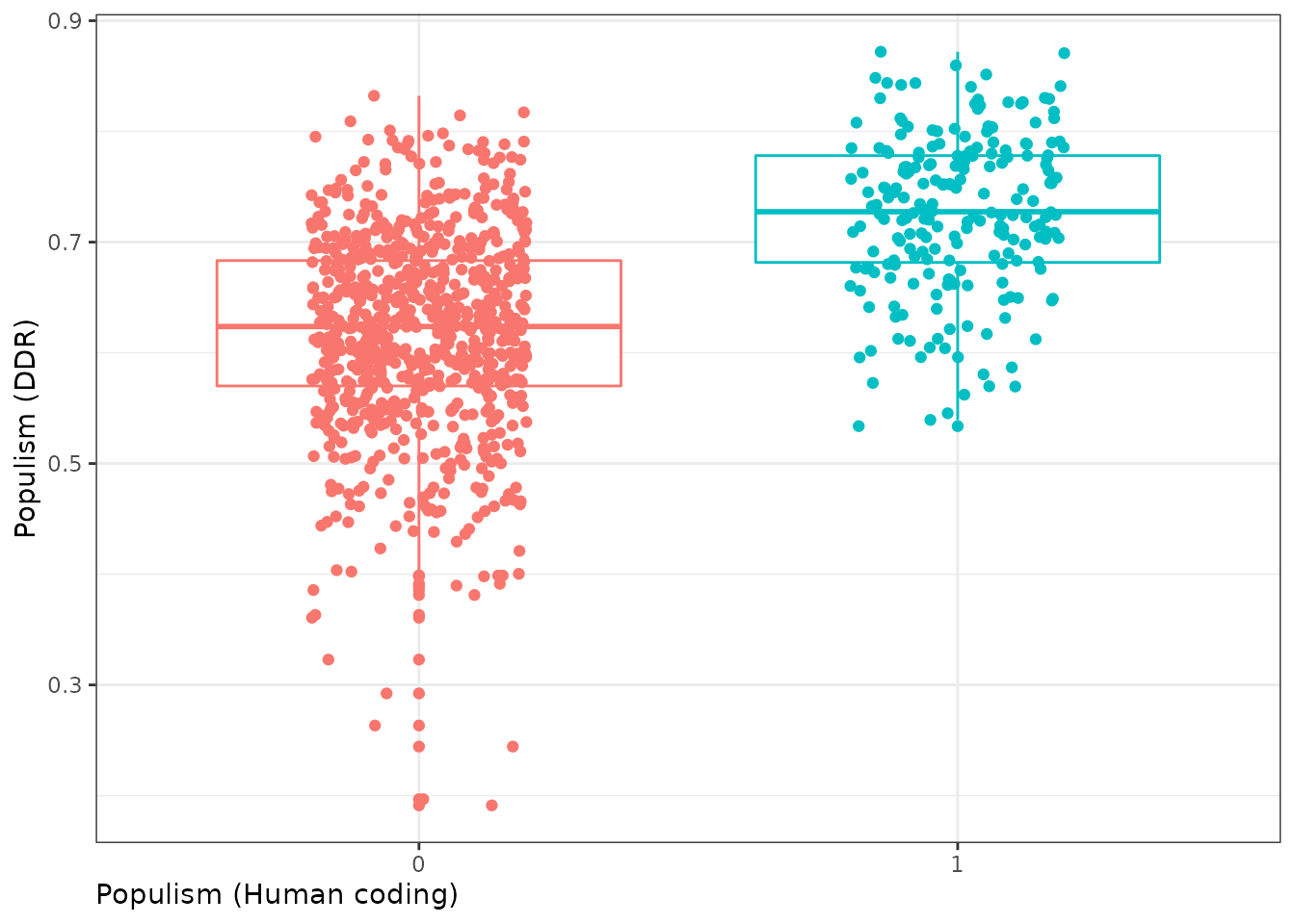
We see that some non-populist Tweets score higher than they should, but the mean populism score for both groups is clearly different - as indicated by the boxplots.
We can also use the parallel-coded 90 Tweets to get some visual evaluation for the gradual measurement returned by the DDR method. ‘Populism’ in the annotated dataset was coded as two distinct categories, anti-elitism and people-centrism. To obtain some gradual score, we just calculate the sum of the coding of these two categories by the two coders, resulting in a score that ranges from 0 to 4. We plot it against the DDR score:
parallel_df <- tw_annot %>%
  filter(rel_test == 1) %>%
  mutate(pop_cum = ppc_A + ppc_B + ane_A + ane_B)


ggplot(parallel_df, aes(x = pop_ddr, y = pop_cum))+
  geom_jitter(height = .1,
              width = 0)+
  geom_smooth(method = lm, se = T)+
  coord_cartesian(ylim = c(0,4))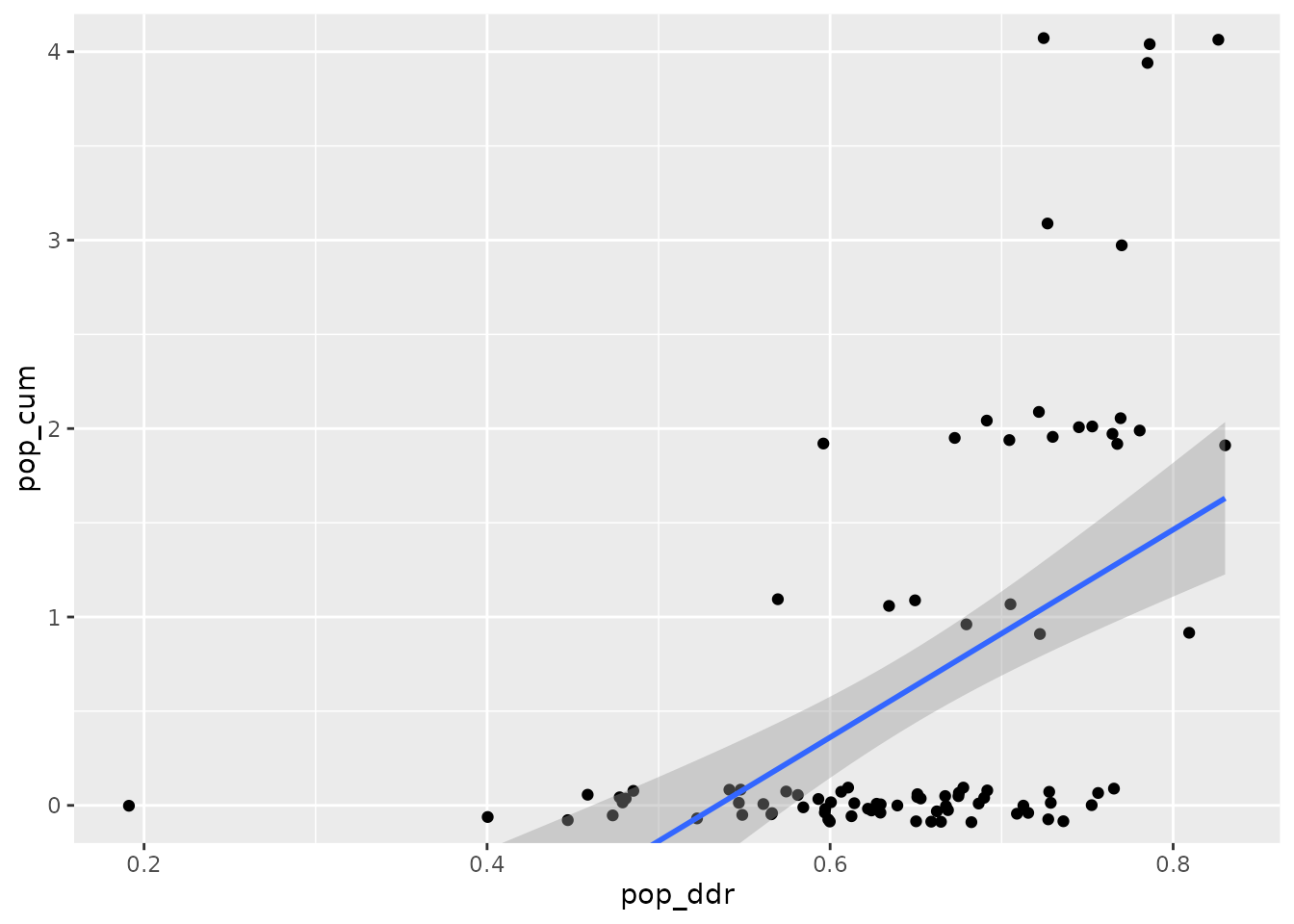
The two (semi-)continuous scores have a Pearson’s r correlation of .53:
cor(parallel_df$pop_cum, parallel_df$pop_ddr)
#> [1] 0.521855
Finally, to assess external validity of our measurement, we compare it on a aggregated level to the POPPA expert rating of political parties (Meijers and Zaslove, 2020). This expert survey provides a gradual rating of populism for political parties. The score is already merged to the tw_data.
# aggregate on party level
tw_party <- tw_data %>%
              group_by(party) %>%
              summarise(pop_ddr = mean(pop_ddr),
                        poppa_populism = mean(poppa_populism))


ggplot(tw_party, aes(x = pop_ddr, y = poppa_populism, label=party))+
  geom_point(na.rm = T)+
  geom_smooth(method = lm)+
  geom_text(hjust=0, vjust=0)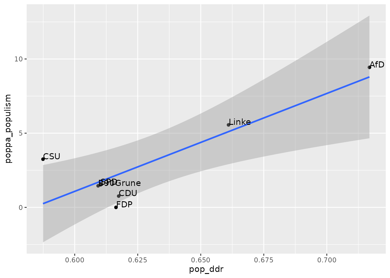
On an aggregate level, the expert ratings of populism for the political parties align very well with the DDR score for populist communication.
Indeed, both scores are strongly correlated:
cor(tw_party$pop_ddr, tw_party$poppa_populism)
#> [1] 0.8667536
Simple visual analysis
The resulting DDR scores could be used, e.g. to investigate temporal shifts in the strategies of the political parties. Below we plot the mean populism score per party over time. We see that the ‘AfD’ clearly is the most populist party, followed by ‘Die Linke’, which is theoretically plausible. We note a sudden decrease of populist communication for ‘Die Linke’ and other parties in August 2020, which could be driven by the growth of a populist coronasceptic movement - which was opposed by all parties but the ‘AfD’. At the end of the timeframe, shortly before the German General Elections in September 2021, the level of populism rises notably for the ‘AfD’.
tw_data %>%
    mutate(day = as.Date(created_at)) %>%
    group_by(party, day) %>%
    summarise(pop_ddr = mean(pop_ddr)) %>%
    ggplot(aes(x = day, y = pop_ddr, color = party))+
    geom_smooth(method = 'loess', span = 0.15, se = F)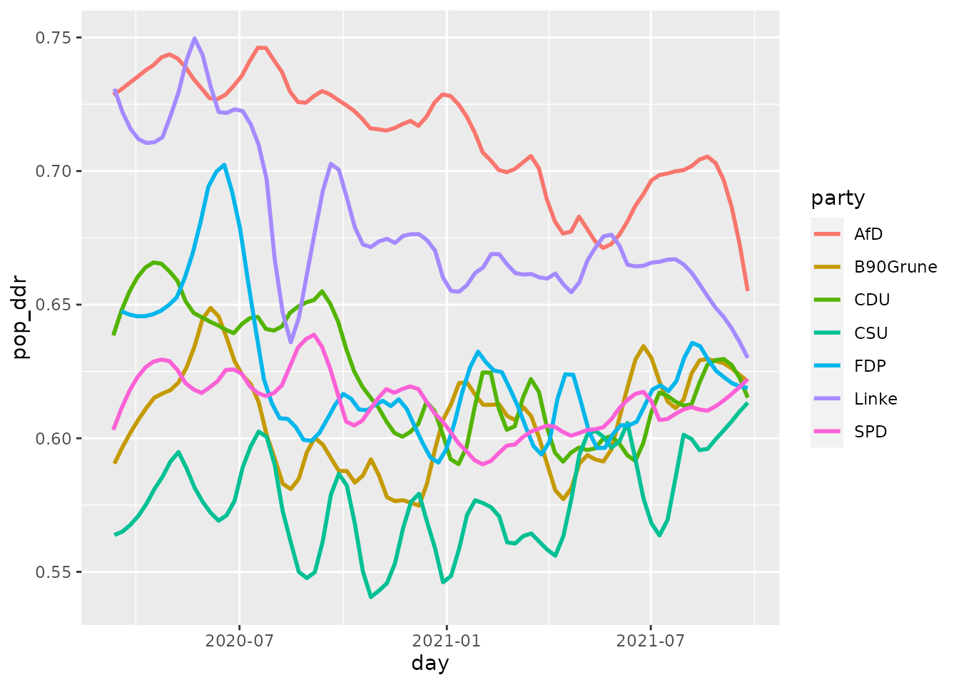
Conclusion
Summing up, the dictionary and measurement produced in this vignette does a good job in differentiating levels of populism in the communication of political parties, on an aggregate level. It also produces somehow plausible results when compared to the cumulative coding of the two coders. And it performs OK when compared directly to the binary hand-codings of Tweets.
However, there is much room for improvement. Here are some possible ways to improve the measurement:
Improve the fastText model by using a much larger training dataset. Pre-trained models are trained on millions of sentences, for example. However, unlike those generic models, you may want stick with material from the specific context (here: communication of political elites).
Improve the fastText model by parameter tuning. E.g., donsider increasing the number of dimensions (
dim, 100-300 are popular choices), increasing the number of epochs (epoch), play around with different ngram lengths (minn,maxn), and play around with the window size for context (ws). You can useget_nnfor face validity plausibility checks, or use a more formal test (e.g., analogy tests) to determine the quality of your fastText model.Use a larger annotated sample for finding good keywords and evaluating their quality. The larger this sample, the lower the risk of overfitting your short dictionary to a too specific context.
Play around with different thresholds in
remove_similar_terms. This function can have a quite dramatic effect of the words included or excluded.Think of a theory-driven, explicit coding-scheme for hand-picking words from the narrowed down subset.
Allow for more combinations per length and dimension (
limit) inget_combis.
Good luck!
References
Bojanowski, P., Grave, E., Joulin, A., & Mikolov, T. (2017). Enriching Word Vectors with Subword Information. ArXiv:1607.04606 [Cs]. Retrieved from http://arxiv.org/abs/1607.04606
Chinchor, N. (1992). MUC-4 evaluation metrics. Proceedings of the 4th Conference on Message Understanding, 22–29. USA: Association for Computational Linguistics. https://doi.org/10.3115/1072064.1072067
Garten, J., Hoover, J., Johnson, K. M., Boghrati, R., Iskiwitch, C., & Dehghani, M. (2018). Dictionaries and distributions: Combining expert knowledge and large scale textual data content analysis. Behavior Research Methods, 50(1), 344–361. https://doi.org/10.3758/s13428-017-0875-9
Grimmer, J., & Stewart, B. M. (2013). Text as data: The promise and pitfalls of automatic content analysis methods for political texts. Political Analysis, 21(3), 267–297. https://doi.org/10.1093/pan/mps028
Meijers, M., & Zaslove, A. (2020). Populism and Political Parties Expert Survey 2018 (POPPA) (Data set). Harvard Dataverse. https://doi.org/10.7910/DVN/8NEL7B
Thiele, D. (2022, June 27). “Don’t believe the media’s pandemic propaganda!!” How Covid-19 affected populist Facebook user comments in seven European countries. Presented at the ICA Regional Conference 2022. Computational Communication Research in Central and Eastern Europe, Helsinki, Finland. Retrieved from https://ucloud.univie.ac.at/index.php/s/PzGzChXroLCXrtt